Arrays¶

Creating vectors¶

To create a row vector, type the elements with a space or a comma between the elements inside the square brackets:

>> x=[1 2 3 4], y=[5,6]

x =

     1     2     3     4
y =

  5     6

>> whos
  Name      Size            Bytes  Class     Attributes
  x         1x4                32  double
  y         1x2                16  double

In the above example, we have created two vectors:

$x = \begin{bmatrix} 1 & 2 & 3 & 4 \end{bmatrix},\quad y = \begin{bmatrix} 5 & 6 \end{bmatrix}$

Hence, when we use whos command, which gives us the information of all variables in the memory, it tells us $x$ has size 1 by 4 and $y$ has size 1 by 2.

The following example shows us how to create a column vector. We enter the elements with a semicolon between them and type the square brackets on the left and right:

>> z=[3;5;7;9]
z =
     3
     5
     7
     9
>> whos z
  Name      Size            Bytes  Class     Attributes
  z         4x1                32  double

Using whos command followed by a name of variable, will give us only the information of that variable. Here the vector z is 4 by 1.

Creating a vector with constant spacing¶

A vector in which the first element is x0, the last element is xn and the number of elements is n is created by typing the linspace command:

>> x=linspace(2,10,5)

x =

     2     4     6     8    10

Another way to create a vector with a constant spacing is to type the first element, follow by a colon (:), the specified stepsize, colon, and then the last element. This way, the number of elements vary upon the chosen stepsize:

>> x=0:0.5:3

x =

         0    0.5000    1.0000    1.5000    2.0000    2.5000    3.0000

Note that the linspace and the above example return a row vector.

Creating matrices¶

A matrix is created by typing the elements, row by row, inside square brackets []. For example, we assign a matrix to variable x:

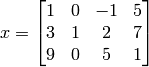
$x = \begin{bmatrix} 1 & 0 & -1 & 5 \\3 & 1 & 2 & 7 \\ 9 & 0 & 5 & 1 \end{bmatrix}$

This can be done by typing the left bracket [, then type the first row separating the elements with spaces (or commas) and type the right bracket ] at the end of last row. Note that a semicolon is typed before a new row is entered:

>> x = [1 0 -1 5 ; 3 1 2 7 ; 9 0 5 1 ]

x =

     1     0    -1     5
     3     1     2     7
     9     0     5     1

Special matrices¶

The zeros(m,n) and the ones(m,n) commands create a matrix of size m by n, in which all the elements are the numbers 0 and 1, respectively. The eye(n) command creates an identity matrix of size n:

 >> A=zeros(2,3)
        A =
     0     0     0
     0     0     0

>> B=ones(3,4)
        B =
     1     1     1     1
     1     1     1     1
     1     1     1     1

>> C=eye(3)
        C =

     1     0     0
     0     1     0
     0     0     1

The rand command generates uniformly distributed numbers iwth values between 0 and 1. The command can be used to assign these numbers to a scalar, a vector, or a matrix:

>> rand

ans =
    0.9058

>> rand(2,3)

ans =
    0.9157    0.9595    0.0357
    0.7922    0.6557    0.8491

>> rand(2)

ans =
    0.9340    0.7577
    0.6787    0.7431

Of course, you will not obtain the same values as given above, since rand generates the numbers randomly. Another similar command is randn which generates random numbers that has Gaussian (Normal) distribution with mean 0 and variance 1. The command randperm(n) generates a row vector with n elements that are random permutation of integers ` through n:

>> randperm(4)

ans =
     4     2     1     3

Indexing techniques¶

For a vector named x, x(k) refers to the element in position k:

>> c=[5 7 2 1 8 3]; c(3)

ans =
        2

In this example, x has 6 elements. If we refer to the index that exceeds the dimension, MATLAB will return an error:

>> c(9)
??? Index exceeds matrix dimensions.

Also note that in MATLAB, the index starts from 1 (unlike some language that starts from 0). The first and the last element of a vector can be refered by c(1) and c(end).:

>> c(0)
??? Subscript indices must either be real positive integers or logical

>> c(1)

ans =
     5

>> c(end)

ans =
     3

A single vector command, c(k) can be used just as a variable. For example, it is possible to assign a new value of only one element of a vector. This is done by typing: c(k) = value:

>> c

c =

     5     7     2     1     8     3

>> c(2)=-1

c =

     5    -1     2     1     8     3

>> c(2)+c(4)

ans =

    0

For a matrix assigned to a variable A, A(m,n) refers to the element in row m and colomn n. Also, just like the vectors, a single element can be used as a variable in mathematical expressions and functions:

>> A=[2 -7 8 1 2 4;0 2 4 5 -3 1;9 9 -6 4 3 1]

A =

     2    -7     8     1     2     4
     0     2     4     5    -3     1
     9     9    -6     4     3     1

>> A(2,3)

ans =
     4

>> 2^(A(1,5))-A(3,2)/3

ans =

  1

Using a colon :¶

For a vector

Command	Refer to
`x(:)`	all the elements of the x
`x(m:n)`	elements m through n of x

For a matrix

Command	Refer to
`A(:,n)`	the elements in all the rows of column n
`A(n,:)`	the elements in all the columns of row n
`A(:,m:n)`	the elements in all the rows between columns m and n
`A(m,n,:)`	the elements in all the columns between rows m and n
`A(m:n,p:q)`	the elements in rows m through n and columns p through q
`A(:)`	vectorize the matrix A into a vector

Using the matrix A from the previous example, we can demonstrate the use of colon as follows:

>> B=A(:,3:5)

B =

     8     1     2
     4     5    -3
    -6     4     3

>> C = A(1:3,4:5)

C =

     1     2
     5    -3
     4     3

It is possible to select only specific elements of a vector by typing the selected elements inside brackets:

>> x

x =

     5    -1     2     1     8     3

>> u = x([5 2 end])

u =

     8    -1     3

In the above example, we wanted to select only the 5th, the second and the last elements of x, and arrange them into a new vector u.

Similarly, to select specific rows and columns of a matrix, we type the selected rows and columns inside brackets, as shown below:

>> D = [10:-1:4; ones(1,7); 2:2:14; zeros(1,7)]

D =

    10     9     8     7     6     5     4
     1     1     1     1     1     1     1
     2     4     6     8    10    12    14
     0     0     0     0     0     0     0

>> F = D([1,3], [1,3,5:7])

F =

    10     8     6     5     4
     2     6    10    12    14

The above example shows how to create a matrix D as a stack of 4 row vectors. The matrix F is created from the 1st and 3rd rows, and the 1st, 3rd, and 5th through 7th columns of D.

Deleting and Adding Elements¶

A single element of a vector, or a range of elements of a matrix, can be deleted by assigning a null value ([ ]). The resulting vector, or matrix will have smaller size. Examples are:

>> y = [8 4 2 4 1 0]

y =
     8     4     2     4     1     0

>> y(4)=[]

y =
     8     4     2     1     0

>> y(2:4)=[]

y =
     8     0

In the first example, a vector y of size 1 by 6 was created. Then we removed the 4th element and y becomes a vector of size 1 by 5. The last expression was to remove the 2nd through the 4th elements of y. The next example shows how to delete elements in a matrix:

>> Z = [22 34 11 6;2 3 4 0;-1 4 7 -9]

        Z =

    22    34    11     6
     2     3     4     0
    -1     4     7    -9

>> Z(:,[1 4]) = []

Z =
    34    11
     3     4
     4     7

>> Z(3,:) = []

Z =

    34    11
     3     4

Similarly, we created a matrix of size 3 by 4. First we removed all rows corresponding to the 1st and 4th columns of Z. Then we deleted all columns corresponding to the 3rd row of Z.

A vector can be made longer by assigning values to the new elements. For example, a vector has 4 elements and we add elements 5,6,...,10:

>> y = [1 3 5 8]; y(5:10)=3:2:14

y =
     1     3     5     8     3     5     7     9    11    13

If a vector has n elements and a new value is assigned to an element with address of n+2, or larger, MATLAB assigns zeros to the elements that are between the last original element and the new element:

>> z = [1 3]; z(5) = 9

z =
     1     3     0     0     9

Rows and columns can be added to an existing matrix by assigning new values or by appending existing variables. For example, we add a new row to the matrix E:

>> E = [1 2 3;4 5 6]

E =
     1     2     3
     4     5     6

>> E(3,:) = [17 31 45]

E =
     1     2     3
     4     5     6
    17    31    45

Now we define a new matrix with the same number of rows as E, and concate it to E:

>> K = -ones(3,2); S = [E K]

S =

     1     2     3    -1    -1
     4     5     6    -1    -1
    17    31    45    -1    -1

S becomes a matrix of size 3 by 5 now. If a matrix of size m by n is assigned a new element with an address beyond its size, MATLAB increase the size to include the new element. Zeros are assigned to the other elements that are added. For example:

>> S(5,9) = 100

S =

   2     3    -1    -1     0     0     0     0
   5     6    -1    -1     0     0     0     0
  31    45    -1    -1     0     0     0     0
   0     0     0     0     0     0     0     0
   0     0     0     0     0     0     0   100

Built-in functions for matrices¶

length(A) returns the number of elements in the vector A:

>> A = [3 4 5 2 4]; length(A)

ans =
     5

size(A) returns a row vector [m,n], where m and n are the size of the matrix A:
```
>> A = [1 3 4;4 5 6]; size(A)

ans =
     2     3
```

reshape(A,m,n) rearrange a matrix A that has r rows and s columns to have m rows and n columns, where r times s must be equal to m times n:

>> A = [1 3 4;4 5 6]

A =
     1     3     4
     4     5     6

>> reshape(A,3,2)

ans =

     1     5
     4     4
     3     6

diag(a) when a is a vector, creates a square matrix with the elements of a in the diagonal:

>> a = [1 2 3]; diag(a)

ans =

     1     0     0
     0     2     0
     0     0     3

diag(A) when A is a square matrix, creats a vector from the diagonal elements of A:

>> A = [1 2 3;4 5 6;7 8 9]

A =
     1     2     3
     4     5     6
     7     8     9

>> diag(A)

ans =
     1
     5
     9

sum(a) when a is a vector, returns the summation of all elements in a:
```
>> a = [1 -2 3 6]; sum(a)

ans =
     8
```

For an m by n matrix A, sum(A,1) returns a row vector whose elements are the summation of all entries in each column. Likewise, sum(A,2) returns a column vector whose elements are the summation of all entries in each row:

   >> A = [1 4;5 6]

   A =
1     4
5     6

   >> sum(A,1)

   ans =
        6    10

   >> sum(A,2)

   ans =
        5
       11

More built-in functions can be explored by typing help elmat.

Examples¶

Function	Description
`mean(a)`	the mean value of the elements of a
`var(a)`	the variance of the elements of a
`max(a)`	the largest element of a
`min(a)`	the smallest element of a
`sort(a)`	arranges the elements of the vector in ascending order
`dot(a,b)`	the scalar product (dot) product of two vectors
`prod(a)`	the product of elements in a
`diff(a)`	the difference between subsequent elements of a

Array operations¶

Addition, subtraction, and multiplication operations in matrices and vectors can be performed by using + - * commands respectively. However, we should keep in mind that the dimension of arrays must agree in any operations:

>> A = [1 2 3;4 5 6], B = [3 4;5 6;7 8], C = [-1 -2 -3]

A =
     1     2     3
     4     5     6

B =
     3     4
     5     6
     7     8

C =
    -1    -2    -3


>> A*B

ans =

    34    40
    79    94

>> A*C
??? Error using ==> mtimes
Inner matrix dimensions must agree.

Transpose operator¶

The matrix transpose operator can be performed by using the single quote (‘) command:

>> A = [1 2 3;4 5 6]

A =

     1     2     3
     4     5     6

>> A'

ans =

     1     4
     2     5
     3     6

Array division¶

The division operation can be explained through the concept of the inverse of a matrix. We say the matrix B is the inverse of the matrix A if

$BA = AB = I$

The inverse of a (square) matrix A is typically written as $A^{-1}$ . In MATLAB, the inverse of a matrix can be obtained by

calling inv(A), or

typing A^(-1):

>> A = [1 2 4;-1 3 9;8 4 2]

A =
     1     2     4
    -1     3     9
     8     4     2

>> inv(A), A^(-1)

ans =

   -5.0000    2.0000    1.0000
   12.3333   -5.0000   -2.1667
   -4.6667    2.0000    0.8333

ans =

   -5.0000    2.0000    1.0000
   12.3333   -5.0000   -2.1667
   -4.6667    2.0000    0.8333

Also note that a (square) matrix is invertible (nonsingular) if and only if its determinant is not zero. Checking the determinant of a matrix can be done by the det command:

>> A = [1 2;2 4]

A =
     1     2
     2     4

>> det(A)

ans =

     0

>> inv(A)

ans =

   Inf   Inf
   Inf   Inf

In this example, the matrix A is not invertible. Calling the inverse function returns Inf which means $\infty$ for each element.

Left division ¶

The left division is used to solve the matrix equation $Ax = b$ . In this equation, x and b are columns vectors and A is a square matrix. If A is invertible, the solution is given by

$x = A^{-1}b$

In MATLAB the above equation can be written by using the left division character A\b.

For example:

>> A = [1 2 4;-1 3 9;8 4 2], b = [-3 5 1]'

A =
     1     2     4
    -1     3     9
     8     4     2

b =

    -3
     5
     1

>> A\b

ans =
   26.0000
  -64.1667
   24.8333

>> inv(A)*b

ans =
   26.0000
  -64.1667
   24.8333

The solution x from \ command is obtained numerically based on the Gauss elimination method, so it is recommended for solving a set of linear equations when large matrices are involved.

Right division /¶

The right division is used to solve the matrix equation $w C = d$ . In this equation $w, d$ are row vectors. The solution of this equation is given by

$w = d C^{-1}$

In MATLAB, the above equation can be performed by the right division command w = d/C:

>> C =[4 2 6;-2 8 10;6 2 3], d = [8 4 0]

C =

     4     2     6
    -2     8    10
     6     2     3

d =

     8     4     0

>> w = d/C

w =

   -1.8049    0.2927    2.6341

>> d*inv(C)

ans =
   -1.8049    0.2927    2.6341

Element-wise operations¶

Element-by-element multiplication, division, and exponentiation of two vectors or matrices is entered in MATLAB, by typing a period in front of the arithmetic operator. This can be done only with arrays of the same size.

.* Multiplication
./ Division
.^ Exponentiation

>> a = [1 2;3 4], b = [-1 4;2 -1]

a =
     1     2
     3     4

b =
    -1     4
     2    -1

>> a.*b

ans =
    -1     8
     6    -4

>> a./b

ans =
   -1.0000    0.5000
    1.5000   -4.0000

Some built-in functions can be performed in an element-by-element fashion. For example, let A be an array. The command sin(A),cos(A), or exp(A) returns an array with the same size as A whose elements are the function values of each element:

>> A = [pi/2 pi/6; pi/4 pi/3]

A =
    1.5708    0.5236
    0.7854    1.0472

>> sin(A)

ans =
    1.0000    0.5000
    0.7071    0.8660

Exercises¶

The length $|u|$ (magnitude) of a vector $u = a \mathbf{i}+ b\mathbf{j}+c\mathbf{k}$ is given by

$|u| = \sqrt{a^2+b^2+c^2}.$

Given the vector 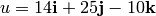$u = 14 \mathbf{i}+ 25\mathbf{j}-10\mathbf{k}$ , determine its length by

defining the vector in MATLAB, and then write a mathematical expression that uses the components of the vector
defining the vector in MATLAB, and then use element-by-element operation to create a new vector with elements that are the square of the original vector. Then use MATLAB built-in functions sum and sqrt to calculate the length.

Two vectors are given:

$u = 10 \mathbf{i}+ 5\mathbf{j}-2\mathbf{k}, \quad v = -6 \mathbf{i}+ 4\mathbf{j}-8\mathbf{k}$

Use MATLAB to calculate the dot product $u \cdot v$ of the vectors. Verify the answer with the command dot (for instruction type help dot).

Use MATLAB to show that the sum of the infinite series

$\sum_{n=0}^\infty \frac{2}{5^n}$

converges to 5/2. Do this by computing the sum for n=50, 500, and 5000. Verify with the result on the infinite sum of a geometric series, which says

$\sum_{0}^\infty a_0 r^n = \frac{a_0}{1-r}$

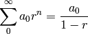
where $|r| < 1$ .

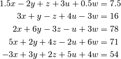
Solve the following system of five linear equations:

$1.5x - 2y +z + 3u + 0.5w &= 7.5 \\ 3x+y - z + 4u -3w &= 16\\ 2x+6y -3z -u + 3w &= 78 \\ 5x + 2y + 4z -2u + 6w &= 71 \\ -3x + 3y +2z + 5u +4w &= 54$

Generate random numbers that are uniformly distributed in a range (-1,4).
Generate random numbers that are Gaussian distributed with mean 1 and variance 4.

Navigation

Table Of Contents