Problems in Engineering¶

Solving linear equations¶

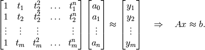
A set of $m$ linear equations with $n$ variables is given by

$\begin{array}{ccc} a_{11}x_1 + a_{12}x_2 + \cdots + a_{1n}x_n &=& b_1 \\ a_{21}x_1 + a_{22}x_2 + \cdots + a_{2n}x_n &=& b_2 \\ \vdots & & \vdots \\ a_{m1}x_1 + a_{m2}x_2 + \cdots + a_{mn}x_n &=& b_m \\ \end{array}$

This can be written in the form of

$Ax = b$

where $A \in \mathbb{R}^{m \times n}, b \in \mathbb{R}^m, x \in \mathbb{R}^n$ .

Case 1: `m = n`¶

When $m=n$ , and if $A$ is nonsingular ( $\det(A) \neq 0$ ), the solution to the linear equations is

which can be obtained by:

x = inv(A)*b

in MATLAB. However, it is recommended to use the left inverse command which is the slash \ sign. This can be done by typing:

x = A\b

This gives the same result as inv command, but the inverse of A is computed in different way (using LU decomposition). Furthermore, if A has a special structure such as symmetric, sparse, or triangular, the \ command provides an efficient algorithm to solve the linear equations. Therefore, to compute the inverse of A, it is recommended to use the following code:

A\eye(n)

where n is the size of A. When A is nonsingular, MATLAB will produce a warning message for both inv and \ commands. For such case, it depends on the vector b whether the equations has a solution or not. For example, let

$A = \begin{bmatrix} 1 & 1 \\ 1 & 1 \end{bmatrix}.$

There there exists a solution if and only if $b \in \mathcal{R}(A)$ (b lies in the range space of A). For example, if $b = [1\; 1]^T$ , then a solution is $x = [1/2 \;1/2]^T$ (and there are many more). However if $b = [1 \; 0]^T$ , then there is no solution x.

if $b \in \mathcal{R}(A)$ , we call the solution $x_p$ that satisfies $Ax_p =b$ as the particular solution. Of course, there are many solutions and they can be characterized by $x = x_0 + x_p$ where $x_0$ lies in the null space of A ( $Ax_0 = 0$ ). A set of vectors that form a basis for the null space of A can be found from the command null:

>> A

A =
     1     1
     1     1

>> null(A)

ans =
   -0.7071
    0.7071

From this example, we read that any vectors lie in the null space of A is a multiple of $[-1 \; 1]^T$ (MATLAB just normalize the vector so that it has a unit norm). We call any vector in the null space of A as a homogeneous solution.

Case 2: `m > n` (overdetermined equations)¶

The matrix A in this case is often referred to as a skinny matrix. When there are more number of equations than the number of variables, it is more likely that the solution does not exist (unless we are really lucky that b happens to be in the range space of A. An example of overdetermined equations that have a solution is

$A = \begin{bmatrix} 1 & -1 \\ 2 & 0 \\ 0 & 1 \\ 1 & 1 \end{bmatrix},\quad b= \begin{bmatrix} 0 \\ 2 \\1 \\2 \end{bmatrix}$

In this example, b happens to be the sum of the two columns of A (in other words, b is in the range space of A). Hence, the solution is $x = [1 \; 1 ]^T$ .

However, very often in practice, when $m >> n$ and $b \notin \mathcal{R}(A)$ , there is no solution to Ax = b. Therefore, we resort to find a solution $x$ that gives $Ax \approx b$ instead. By this approximation, it means Ax is closed to b in a norm-square sense. The solution x that minimizes

$\Vert Ax - b \Vert_2$

where A is a skinny matrix, is called the least-squares solution and denoted by $x_\mathrm{ls}$ . The analytical solution can be obtained by setting the gradient of $\Vert Ax - b\Vert^2$ w.r.t $x$ to zero. This gives

$x_\mathrm{ls} = (A^TA)^{-1}A^T b$

provided that $A$ has full rank. The matrix $(A^TA)A^T$ is a left inverse of $A$ since its multiplication with $A$ on the left hand side gives an identiy matrix. The left inverse can be computed by using pinv command. Hence, with the same example of A given above, but the vector b is $b = [1 \; 0 \; 0 \; 0 ]^T$ . Then there is NO solution to Ax = b, but the least-square solution is:

>> pinv(A)*b

ans =
    0.1667
   -0.3333

Another way to use \ command. It also computes the least-square solution when m > n:

>> A\b

ans =
    0.1667
   -0.3333

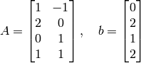
Case 3: m < n (underdetermined equations)¶

In this case, A is a fat matrix. When there are more number of variables than the number of equations, if a solution exists, the solution will not be unique. This can be explained by the following argument. Since A is fat, rank of A is less than or equal to m, and that certainly implies the null space of A is nonzero. Then there will be a nonzero $x_0$ such that $Ax_0 = 0$ . This means if $x$ is any solution to $Ax=b$ then so is $x+x_0$ . A homogeneous solution $x_0$ can be found using the null command. For example,

$A = \begin{bmatrix} 1 & 0 & 1 & 0 \\0 & 1 & 1 & 0 \end{bmatrix}, \quad b = \begin{bmatrix} 1 \\ -2 \end{bmatrix}$

A solution is $x_p = [a \; a-3 \; 1-a \;b ]^T$ where $a,b$ can be any number. Using the null command to find a solution to $Ax_0 = 0$ gives:

>> null(A)

ans =
   -0.5774         0
   -0.5774         0
    0.5774         0
         0    1.0000

Then we read that any linear combination of the above two vectors is a homogeneous solution $x_0$ . So the solutions to Ax=b are not unique and there are infinite number of solutions.

This lead us to consider a solution that has a special property or satisfies some extra conditions. The \ command in MATLAB gives a solution to Ax=b that most entries of x are zero. With the same example of A,b given above, we know that a solution can be written as $x_p = [a \; a-3 \; 1-a \;b ]^T$ (where a,b are free numbers). When we use \ command it gives:

>> x = A\b

ans =
         0
   -3.0000
    1.0000
         0

(MATLAB sets the free variables to zero.)

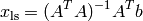
For most cases in practice, we are interested in a solution x that has the smallest size. This means we find $x_\mathrm{ln}$ such that

$\begin{array}{cccc} x_\mathrm{ln} &=& \mbox{argmin} &\Vert x \Vert_2 \\ && \mbox{subject to} & Ax = b \end{array}$

where $x$ is the optimization variable. In other words, we explore a set of solutions to Ax=b and pick the one that has the mininum norm. Such solution is referred as the least-norm solution and denoted by $x_\mathrm{ln}$ . The analytical form of the least-norm solution is given by

$x_\mathrm{ln} = A^T(AA^T)^{-1}b$

provided that $A$ has full rank. The matrix $A^T(AA^T)^{-1}$ is a right inverse of $A$ since its multiplication with $A$ on the right hand side gives an identity matrix. The right inverse is obtained in MATLAB from the pinv command (pseudo inverse). Therefore, the least-norm solution can be computed by:

>> x1 = pinv(A)*b

x1 =
    1.3333
   -1.6667
   -0.3333
      0

We can verify that both the solutions x (from \ command) and x1 (the least-norm solution) solve Ax=b exactly:

>> A*x-b

ans =
   1.0e-15 *

    0.2220
        0

>> A*x1-b

ans =
   1.0e-15 *

   -0.3331
    0.4441

However, in principle x1 must have a smaller norm than x. So, we can check it easily by computing their norms:

>> norm(x)

ans =
    3.1623

>> norm(x1)

ans =
    2.1602

and the result is affirmative.

Another related command in linear albegra is the rank command. It is used to compute the rank of a matrix, which is, by definition, the number of independent column vector of that matrix. For example:

>> A = [1 1 1;2 2 2]

A =
     1     1     1
     2     2     2

>> rank(A)

ans =
     1

Linear least-squares¶

A linear least-squares problem is motivated from solving linear overdetermined equations

$Ax = b$

where $A \in \mathbb{R}^{m \times n } , b \in \mathbb{R}^{m}$ and $m > n$ . In a lot of cases, we cannot solve the equations exactly, so we find a solution $x$ that gives the best approximation of Ax to b instead. Mathematically, we solve

$\mbox{minimize} \;\; \Vert Ax - b\Vert_2^2$

where $x$ is the opitmization variable. To find the analytical solution, we expand the cost objective by

$\Vert Ax - b\Vert_2^2 = x^T A^TA x - 2 b^TAx + b^T b$

Setting the gradient to zero gives

$A^T A x = A^Tb$

Therefore, if $A^TA$ is nonsingular (which is equivalent to A is full rank), then the least-squares solution is given by

$x = (A^TA)^{-1}A^T b$

We do not actually compute the least-squares solution from this expression, but rather use the command A\b. If m=n, the command A\b simply means $A^{-1}b$ , and when m > n, the command A\b produces the least-squares solution.

Curve fitting¶

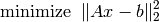
A typical example of least-squares application is a polynomial fitting problem. Suppose we have data points $(t_1,y_1),(t_2,y_2),\ldots,(t_m,y_m)$

Suppose we generate these data sets according to:

>> m = 100; t = linspace(0,10,m)';
>> y = 0.1*t.^3-t.^2+3*randn(m,1);
>> plot(t,y,'x','linewidth',2);

The goal is to fit a polynomial of order $n$ , $f(t) = a_0 +a_1 t + \cdots + a_n t^n$ to these data at the given points $t_1,t_2,\ldots,t_m$ . This is the problem of finding $a_1,a_2,\ldots,a_n$ such that

$\begin{bmatrix} 1 & t_1 & t_2^2 & \ldots & t_1^n \\ 1 & t_2 & t_2^2 & \ldots & t_2^n \\ \vdots & \vdots & \vdots & & \vdots \\ 1 & t_m & t_m^2 & \ldots & t_m^n \end{bmatrix} \begin{bmatrix} a_0 \\ a_1 \\ \vdots \\ a_n \end{bmatrix} \approx \begin{bmatrix} y_1 \\ y_2 \\ \vdots \\ y_m \end{bmatrix} \quad \Rightarrow \quad Ax \approx b.$

Fiting a polynomial of order 1 (an affine function) using the least-squares approach can be done easily by constructing the corresponding matrices A,b by:

b = y;
for n=1:3,
        A = zeros(m,n)
        for k=0:n,
        A(:,k+1) = t.^k;
        end;
x = A\b;
plot(t,A*x,'linewidth',2);
end
legend('data','order 1','order 2','order 3');

(with a change in line style manually.) The result can be shown in the following figure.

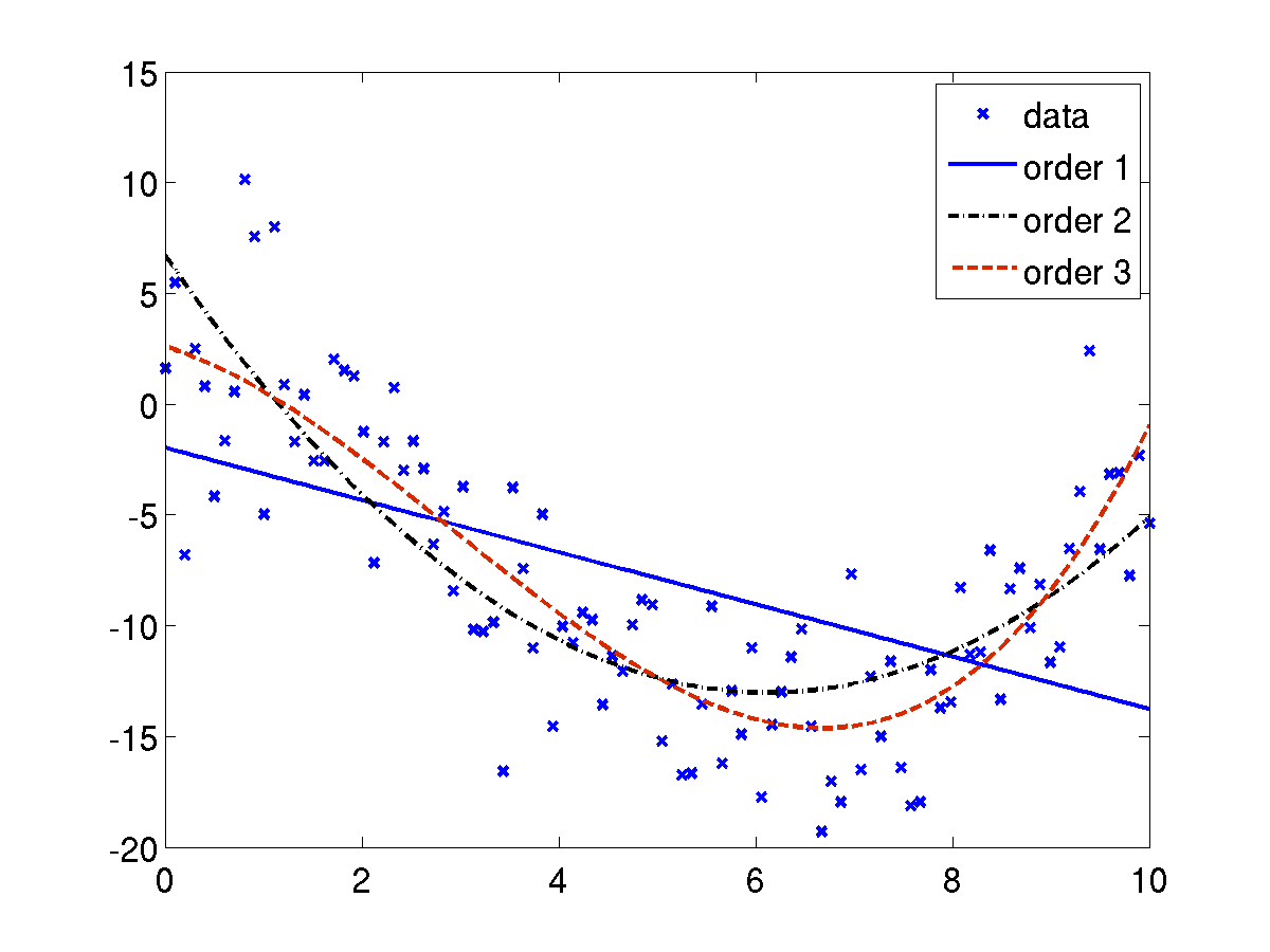
The coefficients of the polynomial for n=3 is kept in the variable x and their values are:

Therefore, the polynomial of order 3 that fits best to the given data points is

$2.6 - 1.38 t -0.75 t^2 +0.085t^3$

Curve fitting problems can be solved with a MATLAB built-in function called polyfit. This command also uses the least-squares method. The basic form of the function is:

p = polyfit(x,y,n)

where

x is a vector with the horizontal coordinate of the data points
y is a vector with the vertical coordinate of the data points
n is the degree of the polynomial
p the vector of the coefficients of the polynomial that fits the data

Let’s try with the same example. Using polyfit to fit a 3rd-order polynomial with the data gives:

>> p = polyfit(t,y,3)

p =
    0.0850   -0.7479   -1.3766    2.5946

This gives the same answer as we had earlier. Notice that the first element of p correspond to the highest power of the polynomial.

In many situations, it is required to fit functions other than polynomials. For example,

$\begin{array}{ccl} y & = & m \log(x) + b \\ y & = & be^{mx} \\ y & = & \frac{1}{mx+b} \end{array}$

In order to apply a least-squares method, we have to write the relation between x and y such that it is linear mapping in the function parameters. For example, the last two functions can be rewritten as

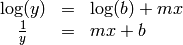
$\begin{array}{ccl} \log(y) & = & \log(b)+mx \\ \frac{1}{y} & = & mx+b \end{array}$

This means that the polyfit can be used to determine the best fit for the parameters $m,b$ .

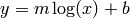For $y = m\log(x)+b$ , use:

p = polyfit(log(x),y,1)

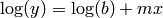For $y = be^{mx}$ or $\log(y) = \log(b)+mx$ use:

p = polyfit(x,log(y),1)

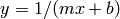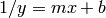For $y = 1/(mx+b)$ or $1/y = mx+b$ , use:

p = polyfit(x,1./y,1)

The result is assigned to p which is a row vector of two elements. The first element p(1) corresponds to m and the second element p(2) corresponds to b.

Exercises¶

The relationship between two variables $P$ and $t$ is known to be:

$P = \frac{5}{m\sqrt{t}+b}$

where $m,b$ are parameters to be determined. The following data points are known: t = 1,2,3,4,5,6,7 and P = 8.9,3.4,2.1,2.0,1.6,1.3,1.2. Determine $m,b$ by solving a curve fitting problem.

A variable $y(t)$ satisfies

$y(t) = K(1-e^{-\lambda t})$

where $K$ is a given constant, and $\lambda$ is the parameter to determined. Given the values of $t,y$ from this data and $K=2$ , use the least-squares approach to find $\lambda$ .

Fit the curve

$f(t) = \frac{1}{1+t^4},\quad -4 \leq t \leq 4$

with a polynomial function of degree $n$ . Vary the values of $n$ and compare the results.

The viscosity of gases are typically modeled by

$\mu = \frac{CT^{3/2}}{T+S}$

where $\mu$ is the viscosity (Ns/m^3), $T$ is the absolute temperature (C), and $C,S$ are empirical constants. Using the data below to determine the constants $C,S$ :

>> T = [-20     0 40 100 200 300 400    500 1000];
>> mu = [1.63 1.71 1.87 2.17 2.53 2.98  3.32 3.64 5.04];

Probability and Statistics¶

A probability density function (pdf) of a random variable can be computed by pdf command which has the form:

>> f = pdf(name,x,A,B,C);

name is the distribution name such as norm (Normal), exp (Exponential), etc.
x is a vector contains all the points at which the pdf is calculated.
A,B,C are parameters associated with the distribution.

For example, evaluating the Gaussian distribution function with mean 1 and variance 2 can be done by:

>> x=linspace(-3,3,100);
>> f=pdf('norm',x,1,2);
>> plot(x,f);

The cumulative distribution function (which is the area under the distribution curve)

$F(x) = \int_{-\infty}^x f(y) dy$

is computed by cdf command which has the form:

>> F = cdf(name,x,A,B,C);

where the input arguments have the same description as the pdf command. The cumulative function must start from 0 and converge to 1 as the value of x increases. For example, we show the cumulative distribution function of a binomial variable with parameters n=10, p = 0.5. This can be done by typing:

>> n = 10; p = 1/2;
>> x = 0:n;
>> F=cdf('binomial',x,n,p);
>> stairs(x,F);

(For discrete random variables, the pdf and cdf are typically plots using stairs command.)

Suppose we have sample values from a given distribution. The histogram of these data should resemble the density function in the long run. For example, we generate 1000 points of Gaussian variables z and a vector x with values starting from -3 to 3. We calculate the histogram of z using the hist command and compare the graphs as described below:

>> x = linspace(-3,3,100);
>> z = randn(1,1000);
>> f = hist(z,x);
>> bar(x,f); hold on;
>> plot(x,pdf('norm',x,0,1);

Optimization¶

A common problem in optimization is to find the solution to

$f(x) = 0.$

The solution $x$ is the value of $x$ where the function cross the x axis. A numerical solution can be obtained by applying an iterative algorithm where the iteration stops when the difference in $x$ between two iterations is smaller than some measure. The function $f$ can be a function of several variables (which means $x$ is a vector.) In general a function can have none, one, several, or infinite number of solutions.

MATLAB provides a built-in function called fzero to compute the roots of a scalar-valued function. It has the form:

x = fzero(function,x0)

x is the solution, which is a scalar
function is the function to be solved. It can be expressed in different ways:
- The function is entered as a string.
- The function is defined as a user-defined function.
- The function is created as an anonymous function.
x0 can be a scalar or a two-element vector. If it is a scalar, it is a value of x near the point where the function crosses the x axis. If x0 is a vector of length two, fzero assumes x0 is an interval where the sign of f(x0(1)) differs from the sign of f(x0(2)). An error occurs if this is not true.
To find a good starting point x0, we can make a plot of the function to check where it crosses the x axis approximately.

For example, let us determine the solution of the equation

$xe^{-2x} = 0.1$

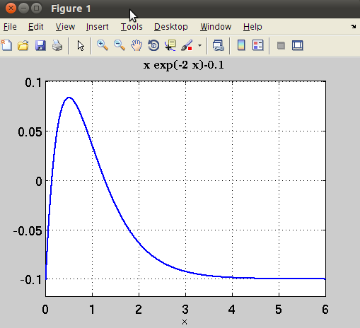
First we plot the function $f(x) = xe^{-2x}-0.1$ :

>> ezplot('x*exp(-2*x)-0.1',[0 6]);grid;

The plot shows that the function has two solutions; one is close to zero, and the other one is between 1 and 2. The first solution can be found by using:

>> x1 = fzero('x*exp(-2*x)-0.1',0.1)

x1 =
    0.1296

We can enter the function description as an anonymous function and find the second root as shown below:

    >> F=@(x)x*exp(-2*x)-0.1

    F =
        @(x)x*exp(-2*x)-0.1

    >> fzero(F,2)

    ans =
1.2713

When the function $f(x)$ is a function of several variables, the roots of the function can be found by using the fsolve command which has the form:

x = fsolve(fun,x0)

where fun is a function that accepts a vector and returns a vector, x0 is an initial point, and x is the solution.

For example, we want to solve the system of two equations and two unknowns:

$\begin{array}{ccc} 2x_1-x_2 &=& e^{-x_1} \\ -x_1 + 2x_2 &=& e^{-x_2} \end{array}$

We can write these equations in the form of $f(x)=0$ as

$\begin{array}{ccc} 2x_1-x_2 - e^{-x_1} &=& 0 \\ -x_1 + 2x_2 - e^{-x_2} &=& 0 \end{array}$

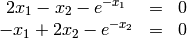
First write the function description as a user-defined function:

  function[F] = myfun(x)
  F = [2*x(1) - x(2) - exp(-x(1));
-x(1) + 2*x(2) - exp(-x(2))];

You must save this function file as myfun.m on your current directory. Next, define a starting point and call fsolve. Make sure that the function $f$ is refered by using @ sign:

>> x0 = [-5; -5];
>> x = fsolve(@myfun,x0);

Equation solved.

fsolve completed because the vector of function values is near zero
as measured by the default value of the function tolerance, and
the problem appears regular as measured by the gradient.

<stopping criteria details>

x =
0.5671    0.5671

Therefore the commands fsolve and fzero can be used to find a solution of an unconstrained optimization problem:

$\mbox{minimize}\;\;f(x)$

since the optimality condition, which is the zero gradient condition:

$\nabla f(x) = 0$

is equivalent to finding the roots of some function.

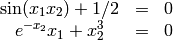
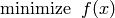
For example, we wish to find the maximum value of the function $f(x) = xe^{-3x}$ for $x \geq 0$ . The plot of this function:

>> ezplot('x*exp(-3*x)',[0 10])

shows that the maximum occurs at a value between 0 and 1. The gradient of this function is $\nabla f(x) = e^{-3x}(1-3x)$ . Therefore, the maximum can be found by:

>> x = fsolve('exp(-3*x)*(1-3*x)',0.5)

Equation solved.

fsolve completed because the vector of function values is near zero
as measured by the default value of the function tolerance, and
the problem appears regular as measured by the gradient.

<stopping criteria details>

x =
    0.3333

MATLAB also provides fminbnd command for finding a local minimum or maximum within a given interval. The command has the form:

[x,fval] = fminbnd(fun,x1,x2)

x is the value where the function has a minimum
fun is the function defined as a string, an anonymous function, or a user-defined function.
x1,x2 is the interval of x.

Within a given interval, the minimum of a function can either be at the boundary of the interval, or at a point within the interval. The fminbnd looks for a local minimum and if it is found, the minimum will be compared with the function values at the boundary of the interval. Then MATLAB will returns the point with the actual minimum value of the interval.

For example, consider the function

$f(x) = x^3-10x^2+20x-32$

on the interval $0 \leq x \leq 10$ , as shown in the figure.

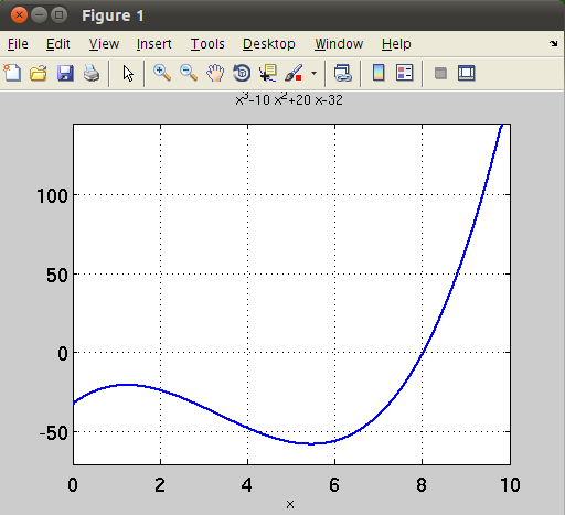
From the figure, a local minimum occurs between 4 and 6. Its location can be found by:

>> F=@(x) x^3-10*x^2+20*x-32;
>> [x,fval]=fminbnd(F,4,6)

x =
    5.4415

fval =
  -58.1468

If we change the interval to [8,10], obviously the minimum must occur at the boundary, which is x=8. Let’s verify by typing:

>> [x,fval]=fminbnd(F,8,10)

x =
    8.0000

fval =
    0.0025

To find a local maximum of this function which occurs at a point between 0 and 2, we must redefine the function F as -F (since maximizing F is equivalent to minimizing -F.):

>> G=@(x) -(x^3-10*x^2+20*x-32);
>> [x,fval] = fminbnd(G,0,2)

x =
    1.2251

fval =
   20.6680

Exercises¶

The Van der Waals equation gives the relationship between these quantities for a real gas by:

$\left ( P + \frac{n^2 a}{V} \right ) \left ( V-nb \right ) = nRT$

where $a,b$ are constants that are specific for each gas. Use the fzero function to calculate the volume of 2 mol $\mathrm{CO}_2$ at temperature of 50C and pressure of 6 atm. For $\mathrm{CO}_2$ , $a=3.59,b=0.0427$ . $R = 0.08206$ is the gas constant. An initial point can be chosen from the ideal gas equation:

$P = \frac{nRT}{V}$

Determine the solution of the equation $10(e^{-0.2x}-e^{-1.5x})=4$ .
Determine the three positive roots of the equation $e^{-0.2x}\cos 2x = 0.15 x^2-1$ .
Determine the positive roots of the equation $x^3-7x^2 \cos 3x +3 = 0$ .
Determine the minimum of the function $f(x) = 10(e^{-0.2x}-e^{-1.5x})-4$ .
Solve the nonlinear equations: