Control System Toolbox
The control toolbox provides algorithms and tools for solving various problems in control system design. This includes analyzing linear systems and controller design. The linear systems can be defined in various formats such as transfer-function, state-space, pole-zero-gain, and frequency-response models. This section will describe elementary tools commonly used in control system analysis and design.
Continuous-time linear systems of order  can be described by a state-space equation
(1)
where  is state variable,
  is the output, and
  is the input of the system. Here we only consider a scalar input scalar output system (SISO), so
  are scalar. The matrix
  is n x n,
  is n x 1,
  is 1 x n and
  is 1 x 1.
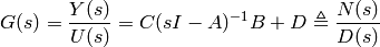
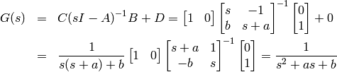
A linear system can also be expressed by a transfer function in s-domain. If we take the Laplace transform of (1) with zero initial condition  , we have

and

Therefore, the transfer function from to is
(2)
The expressions in (1) and (2) are the two typical representations of linear systems. We will show how to write dynamics of a system into these representations.
Consider the dynamic behavior of the liquid level in a manometer tube, responding to a change in pressure, which is given by
(3)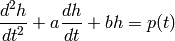
where  is the level of fluid measured with respect to the initial state value,
  is the pressure change, and
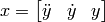
  are constants. To write the dynamic in a state-space format, first we define a state variable (which has two components since the ODE is 2nd-order)
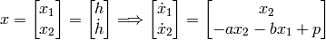
We consider the pressure change  as an input and as the output of the system (
 ). The state-space description of this system is
The transfer function from to is
Of course, we can also obtain the transfer function directly by taking Laplace transform of (3).

In what follows, we consider linear systems in either a state-space format (1) or a transfer function (2). Once we have a system description, we use the Control toolbox to create a system object, and analyze several properties of the system.
Creating LTI objects
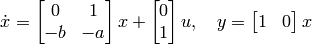
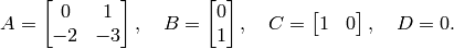
Suppose the constants in example (?) are  , so the matrices
  in the state-space format are
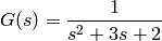
The transfer function is
State-space object
To create a system object in a state-space format, we use the command ss which has the form:
sys = ss(A,B,C,D)
where sys is a state-space object representing the continuous-time state-space model using parameters A,B,C,D. The system in (3) can be created by:
>> A=[0 1;-2 -3];B=[0 1]';C=[1 0];D = 0;
>> sys1 = ss(A,B,C,D)

a =
       x1  x2
   x1   0   1
   x2  -2  -3

b =
       u1
   x1   0
   x2   1

c =
       x1  x2
   y1   1   0

d =
       u1
   y1   0

Continuous-time model.
The variable sys1 has the class of ss object, as can be checked by typing:
>> whos sys1
  Name      Size            Bytes  Class    Attributes

  sys1      1x1              2141  ss
Transfer function
To create a system object in a transfer function format, we use the command tf which has the form:
sys = tf(num,den)
where num,den are the coefficient vectors of the polynomials in numerator and denomenator, respectively. The output sys is a transfer function (tf) object. With the same example, we create the transfer function of (3) by:
>> sys2 = tf([1],[1 3 2])

Transfer function:
      1
-------------
s^2 + 3 s + 2

>> whos sys2
  Name      Size            Bytes  Class    Attributes

  sys2      1x1              2370  tf
Zero-Pole-Gain object
Suppose a transfer function is described by the following format
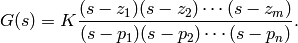
Zeros and poles of a system are defined as roots of the numerator and denominator, respectively. Therefore,  determines the location of zeros and
  are the location of poles. With this representation, the system has gain
  .
.
For example,
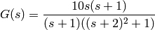
The zeros of  are 0 and -1 and poles of are
  with gain 10. When it is more convenient to specify from the location of zeros and poles, we use the command zpk to create a system object, which has the form:
sys = zpk(z,p,k)
where z,p are vectors containing the location of zeros and poles, respectively, and k is the system gain. Using the above example, the system can be created by:
>> sys3 = zpk([0 -1],[-1 -2+i -2-i],10)

Zero/pole/gain:
     10 s (s+1)
--------------------
(s+1) (s^2 + 4s + 5)

>> whos sys3
  Name      Size            Bytes  Class    Attributes

  sys3      1x1              2528  zpk
Conversion between state-space and transfer function
tf2ss: Convert transfer function parameters to state-space form. The command has the form:
[A,B,C,D] = tf2ss(num,den)
where num,den are polynomials in the numerator and denominator of  , respectively. It returns the
  matrices of a state space representation.
ss2tf: Convert state-space parameters into transfer function form. The command:
[num,den] = ss2tf(A,B,C,D)
returns num,den as the numerator and denominator of where A,B,C,D are matrices of the state-space equation.
Example
Consider a linear ODE
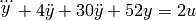
which can be expressed in state-space form as
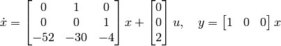
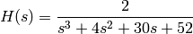
The corresponding transfer function is
First, let’s define the matrices of the state-space equation:
>> A=[0 1 0;0 0 1;-52 -30 -4]; B = [0 0 2]'; C = [1 0 0]; D = 0;
The transfer function can be obtained by:
>> [num,den] = ss2tf(A,B,C,D)

num =
         0   -0.0000    0.0000    2.0000

den =
    1.0000    4.0000   30.0000   52.0000
which agrees with provided above. On the other hand, suppose we define the numerator and denominator of the transfer function as
>> num = 2; den = [1 4 30 52];
then the system matrices in the state-space equation is obtained by:
>> [A,B,C,D] = tf2ss(num,den)

A =
    -4   -30   -52
     1     0     0
     0     1     0

B =

     1
     0
     0

C =
     0     0     2

D =
     0
The result shows that the matrices  are different from those we have derived eariler. This is due to the fact that a state-space description of a system is NOT unique. These A,B,C,D correspond to a choice of state variable
Time-domain analysis
initial: Initial condition response (or zero-input response) of state-space model:
initial(sys,x0,t)
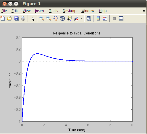
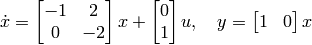
x0 is the initial state vector, t is a final time (or it could be a vector of time samples), and sys is a state-space object. For example, the initial condition response of the system
(4)
where 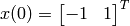 from
from  to
to  is obtained by:
>> A = [-1 2;0 -2]; B = [0 1]'; C = [1 0];
>> sys = ss(A,B,C,0);
>> initial(sys,[-1 1]',10);
impulse: Impulse response of LTI model. We compute a solution of linear systems due to a unit impulse input (
 ) and zero initial condition (). The command has the form:
impulse(sys,t)
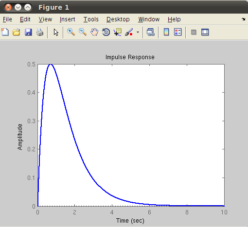
where sys is an LTI object (state-space or transfer function) and t is a final time. For example, the impulse response of system (4) from to is obtained by:
>> impulse(sys,10);
step: Step response of LTI systems. We compute a solution of linear systems due to the unit step input (
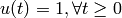 ) and zero initial condition (). The command has the form:
step(sys,t)
where sys is an LTI object (state-space or transfer function) and t is a final time. For example, the step response of system (4) from to is obtained by:
>> step(sys,10);
lsim: Simulate LTI model responses to arbitrary inputs. The command format is:
lsim(sys,u,t,x0)
The vector t specifies the time samples for the simulation and consists of regularly spaced time samples (for example t = 0:0.01:10). The vector u must have as many rows as time samples (length(t)). With the same system given earlier, we can compute the zero-input response (initial condition response) by:
>> t = 0:0.01:10;
>> u = zeros(1,length(t));
>> lsim(sys,u,t,[-1 1]);
The command produces a plot of the zero-input response and the plot must be identical to that of initial(sys,[-1 1]). Now suppose the input is the unit step function. The zero-state response (by setting the initial condition to zero) is done by:
>> u = ones(1,length(t));
>> lsim(sys,u,t,[0 0]);
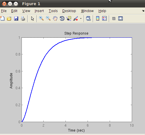
The plot must be identical to that obtained from the command step(sys). Therefore, a response due to an arbitrary input and with a nonzero initial state can be obtained by
>> u = sin(t);
>> lsim(sys,u,t,[-1 1])
(In this example, the input has a sinusoidal wave form.)