Dynamical Systems
Many physical systems are explained by an ordinary differential equation (ODE) and it is often needed to solve for a solution of the differential equation. This solution will explain the trajectory behaviour and characteristics of the system. Some types of ODE can be certainly solved analytically such as linear systems. However, a numerical solution can provide an approximate solution to a general equation. This section, we will show built-in commands in MATLAB used for solving differential equations.
An ordinary differential equation (ODE) has the form:
(1)
where  ,
,  and
and  . An ODE is an equation that contains only ordinary derivatives of the dependent variable. Examples of ODE are
(2)
(3)
(4)
(5)
(6)
If an equation contains partial derivatives with respect to two or more independent variables, then it is called a partial differential equation (PDE). For example, a heat equation
where  is the temperature at a given location
  , and at time
  . Finding a numerical solution of a PDE is an advanced topic. In this document, we will cover how to solve ODE only.
Short review on dynamical systems
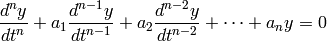
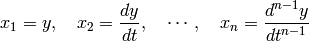
The order of a differential equation is the order of its highest derivative. The systems (2), (3), and (5) are second-order, system (4) is first-order, and system (6) is  -order.
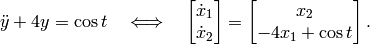
Formulating to a first-order system
Any -order ODEs can be arranged to the form (1) with components in variable , which is referred to as state variable. Consider the system (2). If we define 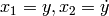 , then
(7)![\ddot{y} + 2y \dot{y} = y^2 \quad \Longleftrightarrow \quad \left [ \begin{array}{l} \dot{x}_1 \\ \dot{x}_2 \end{array} \right ] = \left [ \begin{array}{l} x_2 \\ -2x_1 x_2 + x_1^2 \end{array} \right ].](_images/math/51e28bbc85e94c01621c4cdc01c720a846d0b16d.png)
Similarly for system (3), we define . Then
(8)
The system (4) is already a first-order system with  . For system (5), we define . Then
(9)
Last example is the system (6). Define
then, we can transform (?) into
(10)
Linear systems
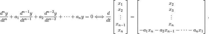
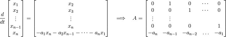
The system of the form (1) is said to be linear or the ODE (1) is a linear equation if  is a linear function in . A linear ODE of order can also be written as
(11)
For example, the systems (4), (9), and (10) are linear systems, while the systems (7) and (8) are called nonlinear systems.
 (identically zero). For example, the linear systems
 Linear systems and examples on chemical processes
Any linear autonomous system can be expressed as
(12)
where  and
and  .
.
Example: Liquid level systems
Suppose  is a steady state liquid flow to a tank and
  is a deviation of inflow rate. Define
  is the deviation of the liquid level in the tank. The differential equation of this system is
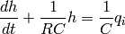
where  are the resistance and capacitance of the tank (parameters of the system). When the inflow rate is zero, this system is autonomous and can be described by the form (12) with
  .
.
Example: Electrically heated stirred tank
Consider a stirred-bank heating system with a mass inflow rate  and an inlet temperature
  . Let
. Let  be the temperature of the tank contents and
  be the temperature of the heating element. The dynamics of the these temperatures are
(13)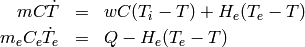
where  are the thermal capacitances of the tank contents and the heating element, respectively. is an input variable,
  is the heat transfer coefficient.
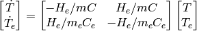
Suppose the input variables  are specified to be zero. Then the system (13) can be formulated to (12) as
Solution to an autonomous linear system
Given an initial condition  . We take a Laplace transform of (12) (elementwise) and we obtain

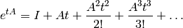
We define the matrix exponential of  as
as
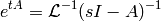
Then the solution to (12) is
Comments
- The matrix exponential
is an
matrix and is a function of
- It is a generalization of
to an
Example
Suppose a linear system is given by
(14)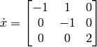
with initial condition  . We simulate a time response of
  from
from  to
to  by:
by:
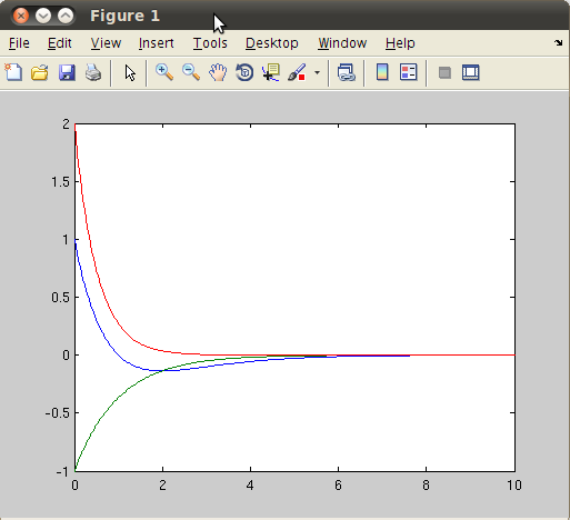
>> A=[-1 1 0;0 -1 0;0 0 -2];
>> t=linspace(0,10,300);
>> x=zeros(3,300);
>> matA = zeros(3,3,300);
>> x0 = [1 -1 2]';
>> for k=1:300, matA(:,:,k) = expm(A*t(k)); x(:,k) = matA(:,:,k)*x0;end;
>> plot(t,x)
We simulate 300 time points, so we must have 300 matrices of  (which is stored in matA). We create a 3-D array matA and for each matA(:,:,k), it is a 3 x 3 matrix of
  .
.
ODE solvers for nonlinear differential equations
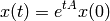
This section provides MATLAB commands used to solve an ODE with the form

for  with a given initial condition
  .
.
An example of a problem to solve is  with
with  . We will explain steps to solve ODE as follows.
1. Create a user-defined function
The description of must be written as a user-defined function (in a separate M-file) or as an anonymous function:
function [dx] = ode1(t,x)

dx = -x^3;
If an anonymous function is used, we can define it in the command window as:
>> ode2 = @(t,x) x^3
Note that though is not an explicit function of , the ODE function must be defined as a function of two variables; time and state respectively.
2. Select an ODE solvers
There are many numerical methods to solve ODEs. Typically, a numerical method starts by dividing the time interval into small time pieces. The solution starts at the known point and the value of at each time step is calculated using an integration method according to the selected solver. A short list of ODE solvers is given by:
ode45, ode23, ode113, ode15s, ode23s, ode23t, ode23tb
The solvers that contain s or t in its name are used to solve stiff problems. We will discuss stiff and nonstiff problems later. For now, we can start by ode45 solver, which can be a good try for most problems.
3. Solve the ODE
An ODE solver command has the form:
[T,X] = solver(odefun,tspan,x0,options)
- Description
- solver is the name of the solver such as ode45, ode23.
- odefun is the function descrption of obtained from step 1.
- tspan is a vector that specifies the interval of the solution
- x0 is the initial value of (the first value of at the first point of the interval.
- [T,X] is the solution of the ODE where T is the time variable.
- options is the structure of optional parameters that change the default integration properties. The options can be set using the odeset function.
For example, we simulate the system with from t = 0 to t=10 by:
>> [t,x]=ode45(@ode1,[1 10],1);
>> plot(t,x);
If we refer to the ODE description written as anonymous function, then we type:
>> [t,x]=ode45(ode2,[1 10],1);
>> plot(t,x);
(without the @ sign.)
We can also solve the ODE in this example analytically. The closed-form solution to is given by
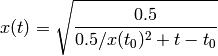
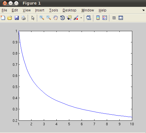
Hence, we can verify if the two methods produce the same results:
>> x0=1
>> y=sqrt(0.5./(0.5/x0^2+t-t(1)));
>> plot(t,y,t,x)
From these steps, a response from the system (14) can be certainly solved from ode45 as:
>> A=[-1 1 0;0 -1 0;0 0 -2];
>> lin1 = @(t,x) A*x
>> [t,x]=ode45(lin1,[0 10],[1 -1 2]');
>> plot(t,x)
The result must be the same as using the expm command obtained previously.
For the rest of this section, we will provide more examples.
Time-varying systems
Given a time-varying system satisfying an ODE

The system can be expressed in a state-space form as
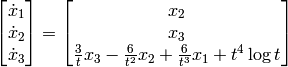
We write the system description in ode3.m as
function dx = ode3(t,x)

dx = zeros(3,1);
dx(1) = x(2);
dx(2) = x(3);
dx(3) = (3/t)*x(3)-(6/t^2)*x(2)+(6/t^3)*x(1) + t^4*log(t);
In this example, the number of state variables is 3, so ode3 must return a column vector of size 3.
We simulate the system from t = 1 to t = 5, with  by
by
>> [t,x] = ode45(@ode3,[1 5],[1 0 -1]');
>> plot(t,x);
Stiff differential equations
Stiffness is ODEs refers to a wide range in the time scales of the components in the vector solution. For example, the following equation may be considered stiff

The closed-form solution to this system is
So the response due to  decays very quickly compared to
  . A numerical solver would need a small step size to compute the rapid changes due to the fast mode. Hence, some numerical procedures that are quite satisfactory in general will perform poorly on stiff equations.
MATLAB also provides stiff solvers such as ode15s, ode23s, ode23t, ode23tb. Consult MATLAB help for detail of each solver.
As an example of a stiff system, we consider the van der Pol equations in relaxation oscillation
for  . To simulate this system, create a function vdp containing the equations:
function dy = vdp(t,y)
global mu

dy = zeros(2,1);    % a column vector
dy(1) = y(2);
dy(2) = 1000*(1 - y(1)^2)*y(2) - y(1);
We solve on a time interval of [0 3000] with initial condition vector [2 0] at time 0:
>> global mu
>> mu = 1000;
>> [t,x] = ode15s(@vdp,[0 3000],[2 0]);
>> plot(t,x(:,1),'-o')
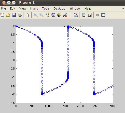
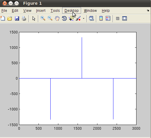
We have solved using a stiff solver ode15s. Then we plot the first component of vector x which is the variable y. If we plot the second component of x, we will see a rapid change in the response:
>> plot(t,x(:,2));
In this example, if we were try to solve using a nonstiff solver such as ode45, the solver would take a long time to complete the task.
Phase portrait
A second-order time-invariant system is represented by
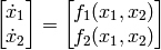
We are interested in a plot of solution  versus
  for all
  . This curve is called a trajectory or orbit of the system. The family of all trajectories or solution curves (which started by different initial points) is called phase portrait. In control systems, it is used to illustrate qualitative behaviour of a 2-dimensional nonlinear system.
Consider a pendulum system described by
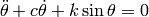
where  are system parameters. Both are positive numbers. So we write the ODE in pendulum file as:
function dx = pendulum(t,x)
global c k

dx = zeros(2,1);
dx(1) = x(2);
dx(2) = -c*x(2)-k*sin(x(1));
Suppose  and we simulate the response from t = 0 to t=20 as
>> global c k
>> c = 0; k = 1;
>> [t,x] = ode45(@pendulum,[0 20],[1 0]);
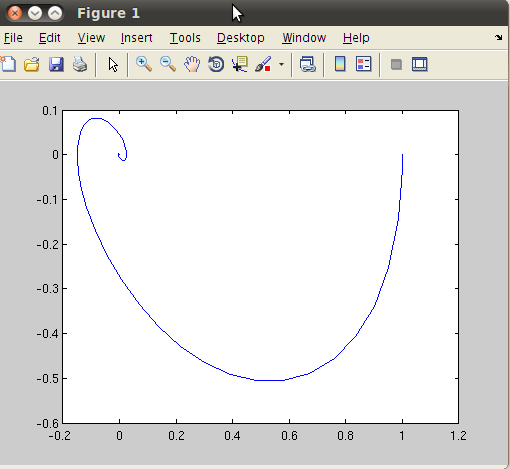
>> plot(x(:,1),x(:,2))
From the plot, the trajectory starts from the initial condition x=(1,0) and then converges to zero. We can make a several curves using different initial conditions by performing a loop:
c = 0; k = 1;
intval = linspace(-1,1,10);

figure;hold on;
for ii=1:10,
for jj=1:10,
        [t,x] = ode45(@pendulum,[0 20],[intval(ii) intval(jj)]);
        plot(x(:,1),x(:,2));
end
end
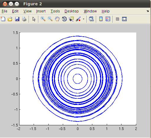
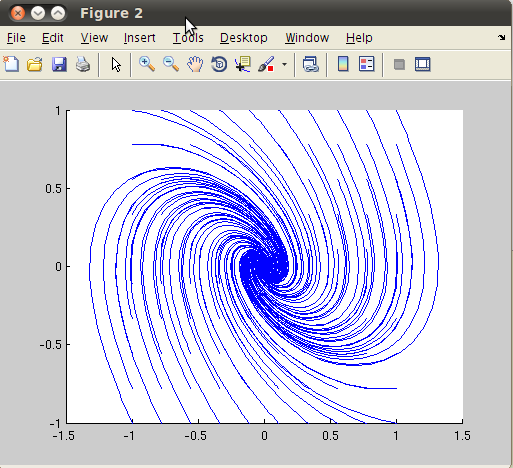
This produces a phase portrait as shown in the figure (left). The trajectories are in a circle shape. Now let  (make c nonzero) and repeat the same process, we have the following plot (right). If
  , it is known that the trajectories eventually converge to the origin (which is the equilibrium point of this system.)
Exercises
- Solve the ODE
using the initial point ![x = [-2 \;\; 3]^T](_images/math/bf45bc3d7034ec6bf5f06d2faa2e936c78efef76.png) .
.
- Solve the ODE from t = 0 to t = 10
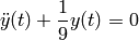
with  .
.
- Solve the ODE from t = 0 to t = 10
with  .
.
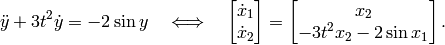
- Solve the Duffing equation
where usually  is small. Plot a phase portrait for both
  and
and  .
.
- Plot phase portraits of the Van der Pol equation using
 . Use different initial points in the interval [-3,3].
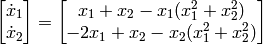
 - Plot phase portraits of the Hopt bifurcation equation
![\begin{eqnarray*}
\dot{x}_1 &=& x_1 [ \mu + (x_1^2 + x_2^2)-(x_1^2+x_2^2)^2] - x_2 \\
\dot{x}_2 &=& x_2 [ \mu + (x_1^2 + x_2^2)- (x_1^2+x_2^2)] +x_1
\end{eqnarray*}](_images/math/8ab575bd1743cf6530878990faf8eb798bcccf6b.png)
for  and
and  .
.
- Compare phase portraits of the three equations
How are the plots related to the poles of the auxillary equations ?