Managing M-files
Many functions are program inside MATLAB as built-in functions, such as sin(x),log(x), etc. These functions can be called by typing their name with an argument input. In programming, there is a need to calculate the value of functions that are not buit-in, that will serve a specific purpose for the users. When a function needs to be evaluated many times for different values of arguments it is convenient to create a “user-defined” function, which can be used just like the built-in functions.
User-defined functions
A user-defined funtion is a MATLAB program that is created by users. The feature of a function is that it has an input and output. The function uses the input data to calculate and return the output. The input and output can be any kind of variables (vectors, scalar, text, etc.)
A simple example of a user-defined function is a function that calculates the time response of a model given by
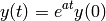
where  is the decay rate,
  the time response at time
  , and
, and  is a given initial condition. In this example, , and are given as input arguments and the value of is the output argument.
Structure of a function file
Function files are created and edited in the editor window.
Function definition line
The first executable line in a function must be the function definition line. Otherwise the file is considered as a script file. The function definition line
- defines the file as a function file
- defines the name of the function
- defines the number of and order of the input and output arguments.
The form of the function definition line is:
function[y] = myfun(x)
where y is the output argument, x is the input argument, and myfun is the function name. The word function, typed in lower case letters, must be the first word in the function definition line. The function name can consist of letters, digits, and the underscore character. The rules for the name are the same as the rules for naming variables.
1. Input and output arguments
Usually, there is at least one input argument, although it is possible to have a function without an input argument. If there are more than one input, the input arguments are separated with commas. The codes within the function file are written in terms of these input arguments and assume that the arguments have assigned numerical values.
The output arguments are listed inside brackets after the word function. If there are more than one output, the output arguments are seperated by comma. In order for the function file to work, the output arguments must be assigned values in the computer program within the function body:
function[y] = myfun(a,y0,t)

y = exp(a*t)*y0;
This example shows that myfun function has 3 inputs and one output. In the body, we use the values of a, t, and y(0) to assign a value to y.
It is also possible that a function has no output argument. For example, a function is used to print some graphs (print), or print a text message (fprintf, disp) to the screen of command window:
function[] = myplot(x)
% x is a vector of length n

n = length(x);
t = 1:n;
plot(t,sin(x.*t));
disp('The plot of e^{-x}sin(x)');
2. Help text lines
Help text line are comment lines (lines that begin with %). They are optional but frequently used to provide information about the function:
function[y] = myfun(a,y0,t)
% function[y] = myfun(a,y0,t)
% myfun computes the time response at time t of the model
%         y(t) = e^(at)y(0)
% The input arguments are a (decay rate),
% y0 (initial condition), and t (time)

y = exp(a*t)*y0;
These information will appear when typing:
>> help myfun
  function[y] = myfun(a,y0,t)
  myfun computes the time response at time t of the model
          y(t) = e^(at)y(0)
  The input arguments are a (decay rate),
  y0 (initial condition), and t (time)
3. Function body
The function body contains the MATLAB code that actually performs the computations. In the function myplot example, the function body is:
n = length(x);
t = 1:n;
plot(t,sin(x.*t));
disp('The plot of e^{-x}sin(x)');
Using a function file
A function file must be saved before it can be used. This can be done by choosing Save as from the File menu in the editior window. It is highly recommended that the file is saved with a name that is identical to the function name in the function definition line. Function files are saved with the extension .m.
A function can be used by assigning its output to a variable as:
>> y = myfun(-0.5,1,10)

y =
    0.0067
or just by typing its name in the command window:
>> myfun(-0.7,2,2)

ans =

0.4932
The input arguments can be a number, or it can be a variable that has an assigned value:
>> a=-0.9; t = 5; y0 = 8;
>> y = myfun(a,y0,t)

y =
        0.0889
Local and global variables
All the variables in a function file are local. This means that the variables are defined and recognized only inside the function file. It is also possible to make a variable common in several function files, and perhaps in the workspace too. This is done by declaring the variable global with the global command that has the form:
global variable_name
- The variable has to be declared global in every function file that the user wants it to be recognized in.
- The global command must appear before the variable is used. It is recommended to enter the global command at the top of the file.
- The global command has to be entered in the Command Window, for the variable to be recognized in the workspace.
- The variable value can be assigned, or reassigned, a value in any of the locations it is declared common.
For example, we create a function file named myfun2.m:
function[y] = myfun2(x)
global b

a = 3;
y = x.^4.*sqrt(a*x+5)./(x.^2+b);
b = 4;
In this example, the local variable is a since it was defined inside the function file, and b was declared as a global variable. This function assigns the value 4 to b every time the function is called. An example of using global variable can be shown as:
>> global b; b = 1;
>> y = myfun2(3)

y =
   30.3074

>> y = myfun2(3)

y =
   23.3134
In this example, we want to assign 1 to b in the command window and use this variable in several function files, so b is declared as global. After calling myfun2, the function computed the output, which is 30.3074 and the function also reassigned the value 4 to b. Therefore, when myfun2 was executed for the second time, the output value has changed to 23.3134, thought the input argument is unchanged.
The example of myfun2.m also shows that we can pass the input x as a vector, since the MATLAB code in the function body also takes care of arithmetic operations for vectors. Therefore, we can compute the function values of several inputs at once:
>> global b; b = 2;
>> x = [3 2 5 1 3];
>> y = myfun2(x)

y =
   27.5522    8.8443  103.5217    0.9428   27.5522
Anonymous Functions
An anonymous function is a simple (one-line) user-defined function that is defined without creating a seperate m-file. It can be constructed in the Command Window or within a script file. An anonymous function is created by typing:
name = @ (arglist) expression
- name is the name of anonymous function.
- arglist is a list of input arguments (independent variables).
- expression consists of a single valid mathematical MATLAB expression.
For example, we create the function myfun3 to compute the function
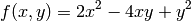
This can be done by:
>> myfun3 = @ (x,y) 2*x.^2-4*x.*y+y.^2

myfun3 =
    @(x,y)2*x.^2-4*x.*y+y.^2

>> myfun3([1 0.5 2],[3 0.9 5])

ans =
   -1.0000   -0.4900   -7.0000
Exercises
Write a user-defined MATLAB function for the following purposes:
Calculate a student’s final grade in a course using the scores from four homework assignments, two quizes, midterm, and final. The grading policy is given by
- Four homework assignments = 10%
- Two quizes = 10%
- Midterm = 40%
- Final = 40%
Each homework and quiz are graded on a scale from 0 to 10. The midterm and final are graded on a scale from 0 to 100. For the function name and arguments use [g,mean,var] = fgrade(R). The input R is a matrix whose elements in each row are the grades of one student. The first four columns are HW grades, the next two columns are the quiz grades, the next column is the midterm grade, and the last column is the final exam grade. The output, g is a column vector with the final grades for the course, where each row is the score of a student. For the last two output arguments, mean and var are the average and variance of student scores.
Give the final grades from the score matrix R given here.